LCC-AMQM
LCC-AMQM consists of three major modules:
Typically life cycle costing, also known as TCO, Total Costs of Ownership, focuses on finding out what your investment will cost during its entire life cycle. LCC will take into account composed interest effects, investments, replacements, maintenance, general costs, production levels, taxes and a myriad of other costs than can be entered manually or using automation.
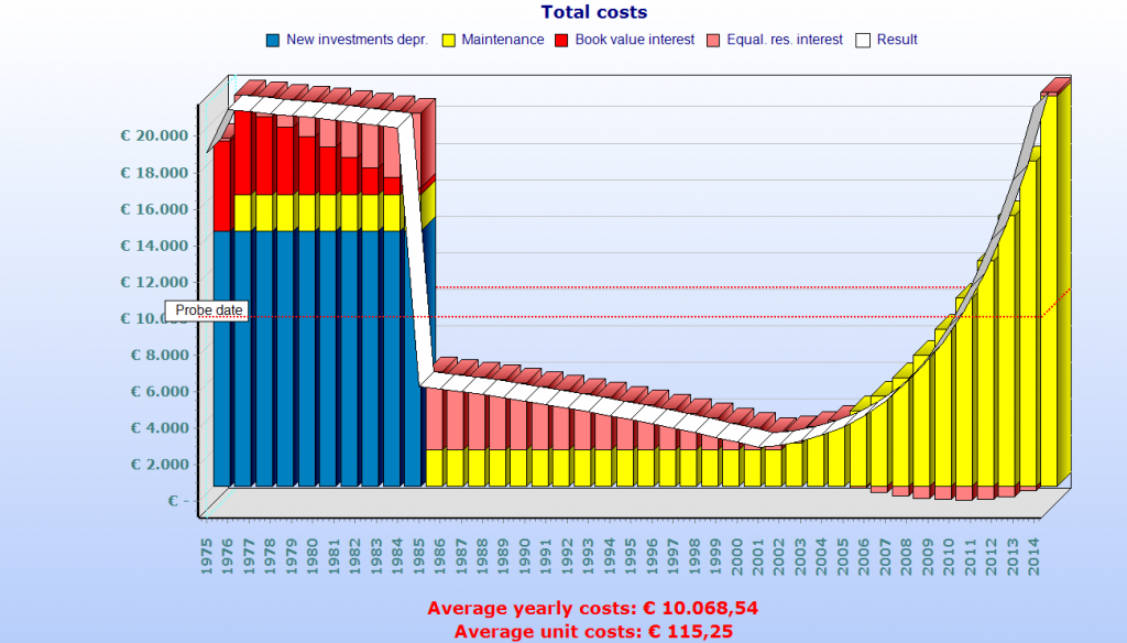
The chart above shows mythical life cycle costing period for a single asset that is expected to last 40 years.
- The first 10 years, costs are high due to interest and depreciations
- Next, follows a lengthy period where only maintenance costs are the main part of the costs.
- After that, closing in on the end-of-life of the installation the installation gets older, maintenance costs raise.
But do assets actually follow this pattern? – the QM analysis tool can tell you this by analysing your recorded CMMS data.
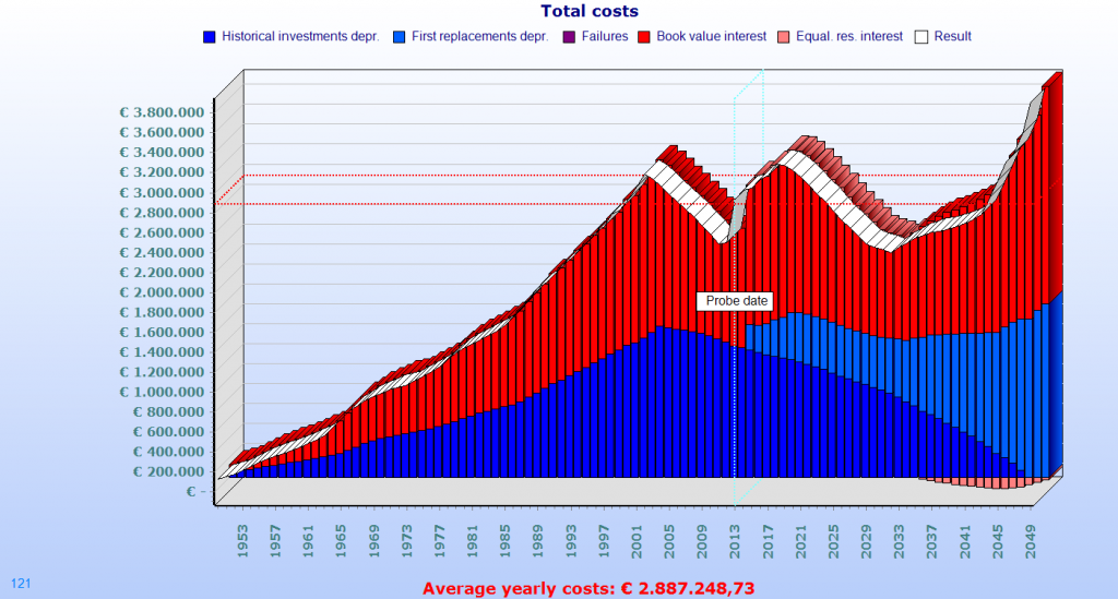
About the chart above, In Europe after WW2, many civil installations were built between 1950 and 1980, and most of the installations are current at “the bottom” of the life cycle curve. But the assets are getting older, their replacement is imminent within the next 20 years. So deciding what assets go first is getting important. Which brings us to the importance of Asset Management, prioritization and budgeting.
Asset Management focuses on knowing what assets you have, and what their condition and importance is. This allows for making the right decision when it comes down to replacing or maintaining assets.
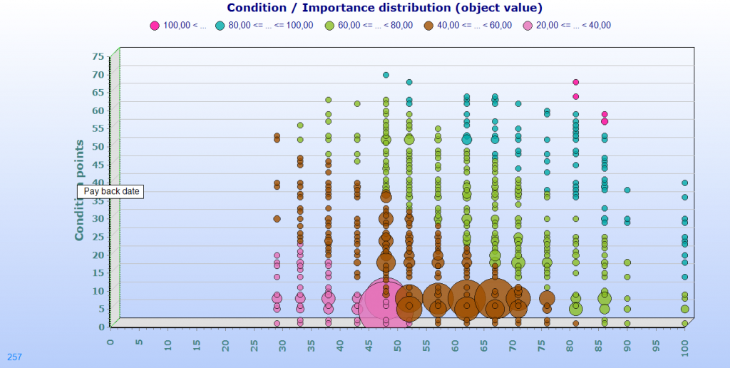
The above chart shows a distribution of assets with their importance and condition points. Colors are in this case assigned per replacement priority band.
Once a priority can be assigned (or calculated) for each asset, LCCAMQM allows to replace them by applying a certain budget for replacements. LCCAMQM allows for using many budgets applicable to many asset groups, which allows to simulate and find the optimum solution for your installations.
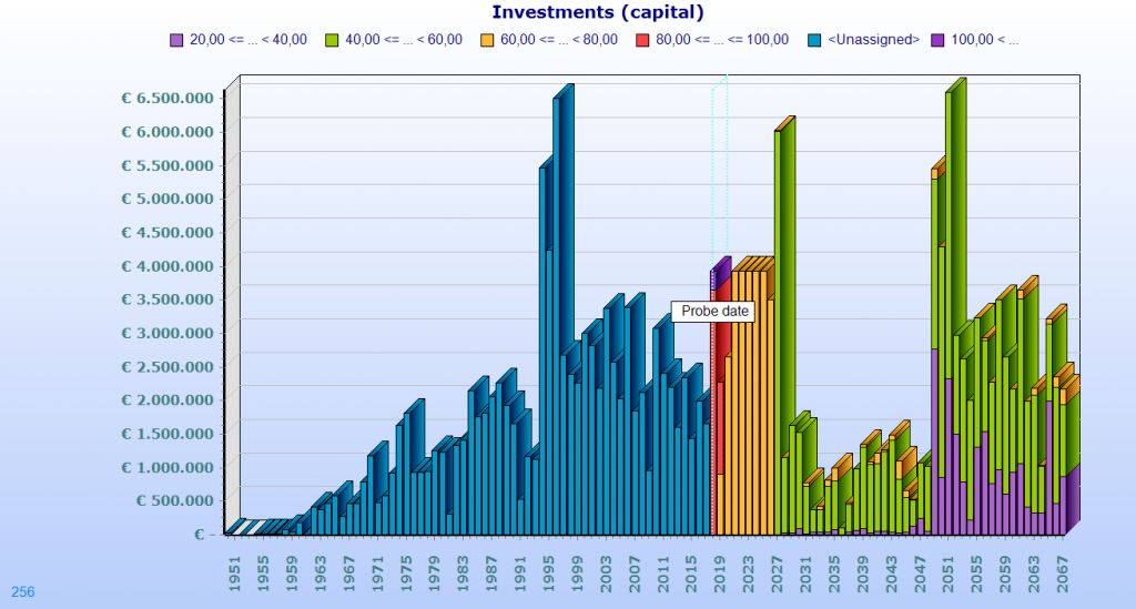
Sample budgeting chart. Replacements are limited to a certain budget, and assets with the highest priority are replaced first. The historical investments are displayed in blue. Budgeting is set up for 2018-2027. LCC-AMQM allows for very fast experimenting with budget amounts and finding out the impact of a certain budget on your average age, predicted failures, depreciations and many other KPI’s that are influenced by this.
Quantitively Maintenance, or better said Quantitative Analysis allows to use the recorded data in your Maintenance management system (CMMS) to provide aging information about your assets and installations. Even when your assets are way older than the recorded data in your CMMS, and your CMMS contains only a few years of data, the life span analysis allows you to find out failure and maintenance behaviour of your assets. Which is often something else then you would expect from the original documentation of your assets.
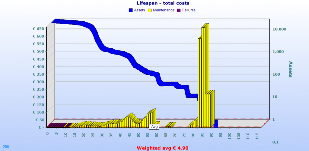
The sample chart above shows an increase of the average maintenance costs during the life span of the assets. The blue line indicates the # of data points available, which is an indicator for the reliability of the data.
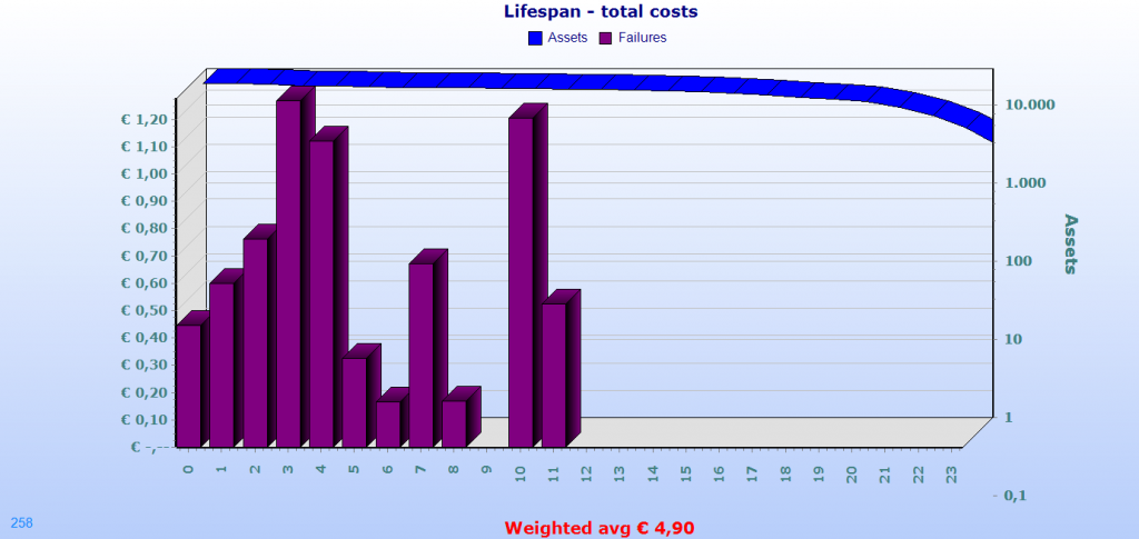
When zooming in on the chart, and hiding the maintenance series, it appears failures have a strong raise in the first few years of these assets, and that failures are either not recorded or don’t take place on assets over 12 years old.
Once the life span data has been determined, and optionally manually evaluated, cleaned and updated, these life span statistical data can be used to perform a projection for each individual asset the future. The established life span curves will be applied to the remaining life span of existing assets, and also for the life span of replaced assets.
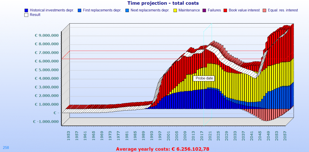
The chart above shows time projection of costs based on life span data statistics and asset replacements.
